Audio amplifier evaluation parameters

Premise

An amplifier, in electronics, is a device that increases the amplitude of an input signal (voltage amplifiers) or increases the amount of current available at the same amplitude (current amplifiers).

An audio amplifier is a voltage amplifier, and so also an ideally constant voltage source.

Unlike amplifiers with different uses, audio amplifiers specialize in amplifying frequencies in the audible range, drive complex loads as speakers and amplify a signal that is not constant neither in amplitude nor in frequency: for these reasons it is necessary to observe many more specifics and parameters in order to describe physically their behavior.

It seems that this is largely forgotten by everyone, probably because first historically and then for marketing issues, the THD parameter has become the one and only concern of those who buy an amplifier.

This also ends up dividing the audio world: some believe they have perfect and impeccable amplifiers only because they have infinitesimal distortions, others have stopped trusting the measurements, since although two amplifiers may have similar levels of distortion, in reality they produce different signals and manage the load differently, resulting in different sounds.

From here, the distortion parameter, for those who trust their hearing, begins to lose importance, until they stop believing that measurements really matter and end up believing in the magic of amazing cables and ground boxes filled with sand.

The main problem lies in education regarding the subject, fortunately the world is slowly becoming more and more scientific and increasingly oriented towards measurements, but the process is really long.

The final point is that a single parameter is not enough to define how an amplifier will behave towards a certain input signal or a certain load at its output.

Amplifier classes

Differently from the household appliances classes, amplifier classes do not define its efficiency, but efficiency is a consequence of the amplifier class operation method and structure.

The class of an audio amplifier defines two things: the method of operation (linear amplification or switching) and the amount of signal amplified (0 to 100%).

The class definition can be applied to a single device (tube, mosfet, transistor, etc ..), to a single stage, or to the entire amplifier.

Class is not synonymous of quality, this only determines some limitations on some parameters, such as efficiency or speed.

Class operation methods

Linear amplification

A linear amplifier uses simple devices, as transistors, tubes or mosfets to directly increase the input signal.

The input signal directly commands the amplification device, that increase the current flow at the output. In a transistor, this is done by adding or subtracting (depends on polarization) current at its base: this cause the electrons flow to increase through the device.

Switching amplification

Switching amplification is a more complex amplification.

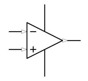
The input signal is summed with an high frequency triangular wave through a comparator, obtaining a square wave with variable duty cycle in function of the input signal.

Then the square wave is linearly amplified with high frequency devices as MOSFETs, and lastly the signal is filtered by a low-pass LC (inductor-capacitor) filter to return the original signal.

Classes

Class A

Class A is the first amplifier class created. The device, or the amplifier stage is always fully-opened: the signal is always within the current flowing through the device or stage.

Due to class amplification method, the efficiency is really low.

Operation method: LINEAR
Maximum efficiency: 25%
Signal conduction: 100%

Class B

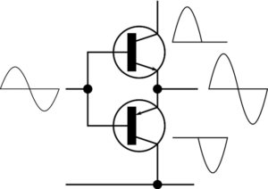
Class B conduct only half of the signal, it was used to greatly reduce the heat generated by class A operation, but it requires minimum two devices to achieve the full conduction of signal.

This permit to open the device only when the signal is put in the input, and so greatly increase the efficiency.

Operation method: LINEAR
Maximum efficiency: 78.5%
Signal conduction: 50%

Class AB

In theory, class B is working fine: when the signal is positive then the upper device is working and when is negative then the upper stop working and the lower device start working.

There is a problem in practice: below a certain voltage threshold, the devices do not conduct. So when the signal approaches the crossing point between the positive and negative parts, there is a period of time where the signal is not conducted. Resulting in the typical distortion called “crossover distortion”.

Consequently, class AB tries to sum class A with B: the devices are kept partially switched on above their minimum non-conduction threshold, below this threshold the signal is conducted entirely (in class A), above this threshold it is conducted partially (in class B).

This greatly reduces crossover distortion, but does not completely eliminate it.

Operation method: LINEAR
Maximum efficiency: 78.5%
Signal conduction: >50% U <100%

Class G & H

Class G and class H were created to maintain the operation method linear and maintaining the same performances, but also to increase efficiency.

The concept is that the devices in class B/AB act as power regulators: the internal area of the signal function is power in output, and everything outer till the supply voltage is dissipated power.

Class G and class H use more power supply rails, to rise the voltage when needed, so the amplifier can achieve theoretically the maximum efficiency.

Operation method: LINEAR
Maximum efficiency: 85.9% (if class G) | >85.9% U <=100% (if class H)
Signal conduction: >50% U <100%

Class D & T

Both class D and T work with the switching mode operation. The reason for using such a complex amplification method is its efficiency. Class D were originally created for pro and PA audio, so a lot of power was needed in tight spaces and with little heat dissipation.

Originally this class had far inferior performances to the linear classes, the biggest problem was a distortion created by the on and off misalignment between the upper and lower devices. This distortion is referred to as “dead time”.

To solve this problem, class T was created, reducing greatly the dead time and increase the synchronization. Later on, the term “class T” disappears, and only class D remains. Today, modern class D reaches performances far superior of medium quality linear amplifiers.

Operation method: SWITCHING
Maximum efficiency: 100%
Signal conduction: 100%

As said previously, amplifier classes are not synonim of quality. But it is really difficult for a switching amplifier to reach it, not in term of signal distortion, or SNR or output impedance, but in term of speed.

The problem is better described below, in the “Slew rate” parameter.

Amplifier parameters

The parameters are divided into two categories: acoustic and non-acoustic.

The acoustic parameters are those necessary to understand how the amplifier behaves with musical signals and its load, and so how is perceived to the human hearing.

The non-acoustic ones instead how the amplifier behaves in its implementation: for example, by connecting a specific power supply to it, or its efficiency, or its stability.

Before we continue, an important statement.

Some say that certain parameters are handled differently by certain classes and that they are not valid in the same way as other classes: this is false. It doesn’t matter the amplification class, and how an amplifier achieves certain performances, but what the load sees and how the amplifier manages the complexity of the load.

[1] Acoustic | Distortion of a fundamental signal (THD)

Distortion is how much an amplifier “dirties” the signal by doing its amplification job.

Distortion of a fundamental is measured inputting a signal of constant amplitude and frequency. By standard, a sinusoidal signal is introduced which has a center frequency of 1kHz. If the amplifier is power amplifier, a non-inductive 8 Ohm resistive load is used to simulate the speaker, if the amplifier is for headphones, the same type of load is used but with 32-600 Ohm impedance.

Distortion is expressed by standard as a percentage, and represents the ratio between the voltage between the fundamental signal and its harmonics generated by the amplifier. The generated harmonics are the byproduct of the amplification job. The higher the harmonics respect to the fundamental signal, the higher the distortion.

This distortion normally rises by about 6dB per octave in linear amplifiers, and with amplitude and frequency in all amplifiers. Also, it rises as the load impedance lowers.

This distortion alone doesn’t say much about the amplifier, but it could tell how it behaves when the load impedance decreases, or if there are crossover distortion problems, if the amplifier is underbiased, correctly biased or overbiased.

On this note, some amp designers and modders boast about turning their amp from class AB to class A by increasing the quiescent current: not a good thing. The stage, or amplifier, must be designed directly in class A in order to work correctly, increasing the quiescent current too much causes the overbiasing effect, ending up increasing the even harmonic distortion.

Acoustically speaking, when the fundamental distortion becomes relevant, there are two audible effects:

If the even harmonics, that is the harmonics in phase with the fundamental, are prevalent, then the signal will be more “sweet” audibly.
If the odd harmonics, ie those not in phase with the fundamental, are prevalent, then the sound will be “shrill” and at times annoying and tiring.

However, this only occurs when the harmonics in question are in the auditory range and “close” to the fundamental. In both cases, the higher the harmonics generated, the less sound quality the amplifier will have.

Disrtotion represent first of all and definitely a degeneration of the initial signal, and therefore the first indicator of an amplifier’s quality.

[2] Acoustic | Intermodulation distortion (IMD)

Intermodulation distortion is measured in the same way as fundamental distortion: it is the result of the ratio between the introduced signal and the harmonics produced. However, in its measurement, two or more signals are introduced simultaneously with the same amplitude but different frequency.

Some signal generators and spectrum analyzers introduce over 10-15 signals simultaneously. The more signals are introduced simultaneously, the more precise the measurement of the intermodulation distortion.

Is important to note here, that for the IMD distortion measurement to be effective, the fundamental signals frequency must be not the same of the possible harmonics frenquency of the other signals. For example, the possibile harmonics for 1kHz are 2kHz, 3kHz, 4kHz etc, if the second signal have the frequency of 3kHz, then it will hide the harmonic amplitude in that position and will offset the measurement (with the second signal harmonics too)

The intermodulation distortion has a high impact on the performance of the amplifier, and is a value indicative of its accuracy.

The validity of this measurement is greater than the simple fundamental, because it makes us understand how the amplifier behaves with a signal close to the musical one. However, all fundamentals are still constant in magnitude.

[3] Acoustic | Thermal and memory distortion

Thermal and memory distortions have nothing to do with the previous ones, despite being measured with a similar method.

To explain how it works, it must be understood that an electronic component varies its performance and parameters as the temperature varies or the signal passes (and then current flows). For example, a resistor varies its nominal value, or a transistor varies its gain or internal resistance.

This type of distortion indicates the quality of an amplifier to maintain its performance as the temperature of the components or the signal varies. The smaller the variation in performance, the less thermal and memory distortion.

A component varies its temperature as the passage of the signal varies, moreover, the thermal error is multiplied by its gain. In fact, it is very important to correct the thermal error where the gain of the stage or component is very high.

Normally, thermal distortion is simulated through temperature sweeps between components. Otherwise, one of the methods to measure it in reality would be to introduce two or more non-regular amplitude signals to the input and verify their output over time.

This parameter strongly determines the enjoyment of the outgoing musical signal. This is the strong point of tube amplifiers, as the gain of the stages is usually very low and the temperature at the passage of the signal is almost constant. However, if a solid-state amplifier is cared for enough, the thermal distortion can certainly be much less than that of tube amps.

[4] Acoustic | Hysteresis distortion

Hysteresis distortion is a type of distortion typical of inductors with magnetic core, for example, it affects the 99.9% of switching amplifiers (class D, T) in commerce and all the linear amplifier who have an output inductor with cores.

It has always been known in the world of electronics and signals, and lately it is much discussed in the world of class D amplification.

The figure above highlights the issue. The signal traverses the B-H curve in each direction as given in the graph. The flux (and thus the voltage) at a specific point on the curve can be different depending how you arrive at that point. For instance, following the path 5 to 7 takes you through point 6, and although points 5 and 7 are identical on the B-H curve, the voltage at that point is not. The same situation occurs when you go from 2 to 4 through 3; the voltage values at identical points 2 and 4 are different depending on the path you took to arrive there. Clearly, there are voltage ‘jumps’ when, after traversing a minor B-H loop, you arrive at the same point at the major loop where you were before. So, there is an element of which causes strong non-linearity.

[5] Acoustic | Damping factor (DF)

The effects of damping factor on the loudspeaker are better described in the article Damping Factor effects on loudspeakers. We invite you to read the full article about the damping factor effects and how it works to better understand.

[6] Acoustic | Slew rate (SR)

The effects of slew rate are better described in the article Slew rate effects on audio. We invite you to read the full article about the slew rate effects and how it works to better understand.

[7] Acoustic | Bandwidth and phase

The bandwidth is nothing more than the frequency response of an electronic object. In the case of an audio amplifier, is measured the output voltage obtained with a signal of constant amplitude at the input but of variable frequency.

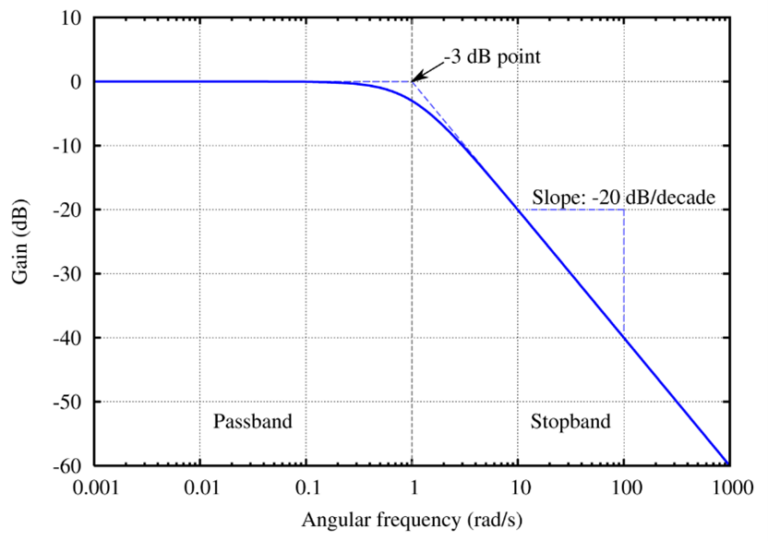
The band is considered the set of frequencies reproducible by the amplifier with the same input voltage. The band extremes are defined when the output voltage (always with the same input voltage) reaches half from the nominal value, that is -3dB point.

The nominal voltage obtained with the same input, on the other hand, is called “gain” and is expressed in decibels. If an amplifier has 27dB of gain it means that it amplifies the input voltage by about 22 times at the given bandwidth frequencies.

The reason the output voltage decreases as the frequency increases is that an amplifier does not have infinite speed. In fact, bandwidth and slew rate are extremely linked to each other: in order to reproduce a frequency with the same voltage, a higher speed is necessary, otherwise the output voltage decreases. For this reason, low-bandwidth amplifiers also have, normally, limited slew rates. (see the Slew rate article or the Power Bandwidth parameter below)

As the frequency increases, with constant speed, the voltage decreases. This means that the current is carried on the load with a delay compared to when it should arrive: the amplifier manages less and less the current requirement of the load as the frequency increases. This creates an effect defined as “phase shift”.

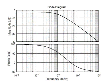
The phase shift of a frequency is a completely normal behavior and is part of every frequency response, regardless of the implementation of the components and independent of the electronic object. In the case of an audio amplifier, a phase change corresponds to a shift of the transient over time.

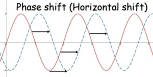
The greater the phase shift, the greater the shift of the transient in time: in practice, the transient experiences a delay in its reproduction with respect to its original position.

This could be a big problem in very small bands: the smaller the band, the greater the phase shift in the audible frequency range. Very large bands are often considered useless in audio, as the upper end is only 20kHz. However, extended bands allow for minimal phase shifts and high slew rates.

In some cases, narrow bands also represent attenuation in the audible range if the slope is too shallow and the cutoff point too close to the audible band.

With a band of only 40kHz there is a phase shift of 40° at 20kHz, with a band of 500kHz there is a shift of only 3° and almost zero attenuation.

The absolute phase would be of little importance if the amplifier were to reproduce a single frequency. However, an audio amplifier must reproduce several frequencies together (musical signal), and if the phase causes a transient to shift a lot, it ends up in the wrong time position relative to the other transients: resulting in staggered playback.

[8] Acoustic | Power bandwidth

Generic bandwidth is normally measured at low input voltage, however power bandwidth is much more important. This is strictly dependent on the slew rate and the load, and unlike the classic band, it varies as the output voltage varies.

The higher the output voltage, the lower the power band: in practice it defines, with the same slew rate, what is the maximum reproducible frequency at a given voltage.

An amplifier could also have a very wide band, but with a low slew rate, it would still not be able to reproduce the entire audible range of frequencies at the specified output power.

See above for a better explanation of the Slew rate parameter.

[9] Acoustic | Signal to Noise ratio (SNR)

The Noise Floor is the output noise of an amplifier when there is no signal at its input, or when its input is connected to ground.

It corresponds to the noise perceived and produced by the speakers when the amplifier is turned on but with no input signal.

SNR is the signal to noise ratio is the noise generated by the passage of the signal, it could increase or in some cases decrease as the input signal increases. Not to be confused with the harmonics generated by the fundamental signal, this ratio always represents the difference in voltage between the fundamental and the generated noise. The higher the SNR, the lower the noise passing through, this means quieter amplifiers: but not necessarily less distorted. In many cases it happens that amplifiers with higher SNRs have more distortions than amplifiers with lower SNRs.

[10] Acoustic | Power factor

The Power Factor is a parameter that defines the real output power of an amplifier at a specific frequency. It is determined by the phase between the output voltage and current. The Power Factor is defined as 1 (full) when the phase between the output voltage and current is equal to 0°.

It is determined not only by the amplifier, but also by the load connected to its output: inductors and passive crossover capacitors always negatively affect it.

The Power Factor plays a fundamental role in the perception of the sensitivity of the bandwidth. It is also and above all diminished by the lack of slew rate and bandwidth, as well as by the lack of damping factor and therefore of the loudspeaker control.

[11] Non-acoustic | Input impedance

The input impedance of an amplifier, being a voltage generator, should be infinite in theory, but in practice it has some problems.

Often this is identified as an audible parameter: in truth, this become audible only if at fault.

If the input impedance is too low, the source may fail to deliver enough current to drive the amplifier input, resulting in damage to the input signal.

If too high it makes the amplifier subject to various disturbances and noises.

For this reasons the input impedance range is normally between 10kOhm and 47kOhm, perfect values for almost every audio source and to mantain the input noise very low.

[12] Non-acoustic | Output maximum voltage

The maximum output voltage refers to the power supply voltage of the amplifier. The higher the voltage the amplifier is powered with, the higher the available output voltage, unless it is internally limited.

[13] Non-acoustic | Output maximum current

The maximum output current refers to the Safe Operating Area (SOA) of the output devices and the supply voltage. The greater the number of output devices, the greater the current available. The lower the supply voltage and the greater the current available, remaining in the SOA.

To remember, that the current is a device-specific property, a single pair of a specific output devices could easily deliver more current than multiple pairs of devices of a different model.

To consider all, unless it is internally limited.

[14] Non-acoustic | Output power

Output power is a complex matter, but still an inaudible parameter.

The output power is a thermal limit, not an operational limit: an amplifier rated 100W can also deliver 500W on the load, but it will heat up much more.

It is about how much power an amplifier can deliver remaining thermally stable, but it can also be limited by supply voltage.

Normally, power is measured by taking the maximum RMS output voltage and finding the current based on the load. This is called “RMS power”, but in electronics it does not exist, and it is also a misconception of power measurement: in this way it means that an amplifier with unlimited output voltage then has unlimited output power, but in reality it doesn’t.

The “RMS”, root mean square, is a property of wave function. The power is not a function, but the integration of voltage with the load impedance: for this reason, “RMS power” does not have any sense mathematically.

For a standard, the Audio Engineering Society (AES) has established the “AES power” or “rated power” parameter, is the power that the device is able to deliver (in the case of an amplifier) or absorb (in the case of a loudspeaker) for at least two consecutive hours without overheating, breaking or going into protection.

This power is totally independent of the load impedance, because it defines the heat dissipation that the amplifier can withstand for long periods of time. The standard also defines as “maximum power” double the “rated power” (+3dB).

Often a higher output power is understood as an amplifier that saturates the signal less. In truth, the saturation or clipping derives solely from the maximum output voltage and slew rate. Most of the time it happens that an amplifier that is able to dissipate more power has a much closer saturation point than one that dissipates less, due to its reduced supply voltage.

As maximum current, AES power or rated power, is referred to the devices SOA and dissipation power of the heatsink.

[15] Non-acoustic | Power supply rejection ratio (PSRR)

The PSRR is also referred to as the Power Supply Rejection Ratio. It is a factor that determines the rejection of disturbances deriving from the power supply, as well as the rejection of noise, also that of ripple.

The greater the rejection, the less the variation of the amplifier performances will be with the variation of the power supply performances.

It is measured by placing the amplifier inputs to ground, and inserting a variable frequency voltage on one of the power supply branches. The greater the attenuation of the signal on the amplifier output, the greater the PSRR. This normally decreases as the frequency rises. Also, an amplifier with a lot of feedback will be less prone to power disturbances, as these will be corrected by the output from the feedback itself.

[16] Non-acoustic | Common mode rejection ratio (CMRR)

The CMRR is the Common Mode Rejection Ratio, it is typical of amplifiers with differential inputs, it measures the tendency of the device to reject the input signals common to both inputs.

It therefore also identifies the amplifier’s ability to reject external disturbances (as EMI), as well as voltage variations and various fluctuations between the differential inputs.

[17] Non-acoustic | Load invariancy

It is the tendency of a well designed amplifier not to vary its performance when the connected load varies, whether this is purely resistive, reactive or capacitive-reactive. Furthermore, it identifies the quality of not varying the performance as its impedance varies.

Ideally, an amplifier is load-invariant.

But in reality there are really a few amplifiers that don’t vary the performances with the load.

The load-invariacy can be observed in the percentage of difference in current between one load and another of different impedance at the same voltage. A perfect doubling of current is never obtained when the impedance of the load is halved at the same output voltage: this is because the amplifier loses efficiency and because the input impedance does not remain constant but increases. Very good amplifiers, they manage to get almost a doubling, others much less.

The damping factor is also an indicative factor of how the amplifier behaves under varying load conditions: low damping means low correction factors and therefore also a large variability.

[18] Non-acoustic | Compensation-Invariancy and amplifier stability

Compensation allows an amplifier to remain stable in the high frequencies. If there were no compensation, the internal devices and stages would be prone to oscillations and free from any restrictions in the reproduction of high frequencies.

Each active device present in the electronic circuits have a maximum band of reproducible frequencies before their break-down. The lack of adequate compensation could lead these devices to deliver as much voltage, current or power as possible (according to their SOA), resulting in a melting or breakage of the devices themselves, especially if power devices.

An adequate compensation design requires the use of adequately positioned poles and specific components: such as the use of NP0 (C0G) capacitors, which do not vary their capacity as the voltage and temperature vary, and which also do not add further distortion.

High frequency stability is linked to three factors: bandwidth and respective phase, slew rate and compensation. A high-speed, wide-band electronic device is more prone to oscillations than a slower, small-band one. However, this is not always said, in fact, often an amplifier with even a reduced band and a low slew, with incorrect compensation, could be far more unstable than one with a much wider band and higher slew, due to peaks in bandwidth and/or phase delays in open loop gain.

A truly stable amplifier, it is with any load. The most difficult load is certainly the capacitive one.

The test is performed (normally) by placing a low capacitance capacitor (1nF) on the output, with no other added. The capacitor, with no resistor in series, will add a peak at the highest frequency of the amplifier bandwidth. The test aims to obtain the output response of a square wave, searching for any ringings and oscillations.

This allows us to understand how the electronic device behaves in the absence of a load, or with very distant loads (where the capacitance of the cable that connects it is very high).

Bands and phase, like the other performances, can vary according to the temperature, the internal variables of the device or, as often happens, to the variation of the load.

Often, as happens in switching amplifiers (class D, T, S, etc), the band varies a lot as the impedance of the load varies. This is because the output low pass filter is calculated on the generic impedance of a specific load.

It is a variable linked to the load-invariancy of the amplifier. Band stability is also linked to high frequency stability. With non-standard loads some amplifiers may have oscillations due to variation and the creation of phase peaks and rotations in the band.

[19] Non-acoustic | Thermal stability

Thermal stability indicates the ability of an amplifier to remain thermally stable, and its propensity not to overheat with consequent thermal drift.

Note that the thermal drift can be both positive and negative. In the case of certain devices, such as lateral MOSFETs, the thermal drift is negative. In contrast, BJT transistors are positive thermal drift devices.

A stable amplifier keeps the temperature constant, and a well-designed one does not change its performance as the temperature changes.

Some amplifiers require an heating-up time to work good, that is clearly a sign of bad design.

It is a factor directly related to memory distortion, the smaller the temperature variation at the passage of the signal, the lower the memory distortion.

[20] Non-acoustic | Open loop gain and closed loop gain

Open loop gain is typical of amplifiers with differential inputs. It is the gain obtained by placing the inverting input towards ground. It determines two things: the amount of correction that is achieved at a specific frequency, and the maximum closed-loop gain available to the amplifier.

Furthermore, it is possible to determine the general high-frequency stability of an amplifier from it, by observing the phase with respect to the gain of the frequency response.

In amplifiers without differential inputs, this is simply referred to as “gain”. Determines the multiplication of voltage that the input signal receives with respect to the output signal. If the amplifier gain is 27dB, for example, the voltage multiplication will be 20 times the input signal.

In differential amplifiers, the gain is decided by a voltage divider placed between the amplifier output and the second differential input. The closed loop gain is necessarily always less than the open loop gain. The higher the gain, the smaller the bandwidth, the lower the gain, the more likely it is that the amplifier will become unstable and the band will have a high frequency peak.

[21] Non-acoustic | Efficiency

Efficiency is the ratio between the absorbed power and the delivered one. Given by the following variables:

Supply voltage versus output voltage: efficiency normally decreases as supply voltage increases, and also is lower when the delta between supply voltage and output voltage is higher
Operation class: depending on the class the amplifier can reach a maximum efficiency
Quiescent current: there is always a dissipated power also when input signal is not present
Load impedance: the efficiency normally decreases as the load impedance lowers

Conclusions

As you can see, the number of parameters to judge an amplifier is not only limited to distortion, SNR and damping factor.

There are many other parameters important as well. Once we know all of them, we can already say how an amplifier will behave with the load, without even listening the setup.